Lesson 2 of 6 · 48 min

Significance & power

p-values, statistical power, the sample-size equation read four ways, and confidence intervals — what each actually means (and what the ASA says it does not), why power is set by variance not effect, and the misinterpretations that end interview rounds and ship bad launches.

One equation, read four different ways

Most of the statistics in A/B testing reduces to a single relationship between four quantities — significance level α, power 1−β, the metric’s variance σ², and the effect size you can detect — and a sample size n that ties them together. Pick any two and the rest are fixed. The senior skill is not memorising the formula; it is knowing which way you are reading it (planning runtime? bounding the effect? checking the test’s power?) and refusing the misinterpretations the American Statistical Association had to publish a formal statement to stamp out. This is the round where a single sloppy sentence — “p = 0.06 means a 6% chance the null is true” — ends the interview.

Start with what a p-value actually is: under the null hypothesis H₀ (no effect), the p-value is the probability of observing a test statistic at least as extreme as the one you got — P(T ≥ t_obs | H₀). For a two-sided z-test, p = 2·(1 − Φ(|z|)). That is the entire definition. The ASA’s 2016 statement (Wasserstein & Lazar) exists because practitioners routinely claim things it does not say: principle 2 — a p-value is not the probability that the hypothesis is true; principle 5 — it does not measure the size of an effect; principle 3 — decisions should not rest on whether p crosses a threshold alone.

The z-test for two means / proportions

For two arms with sample means and sizes n_t, n_c, the estimated treatment effect is Δ = ȳ_t − ȳ_c, and the standardised statistic under the null is Z = Δ / √(σ_t²/n_t + σ_c²/n_c). By the central limit theorem this is approximately standard normal once each arm has roughly ≥1,000 observations and the metric isn’t wildly skewed. For a proportion (conversion) the variance is p(1−p), which is maximised at p = 0.5 — so a metric near a 50% base rate needs the most samples, a counter-intuitive fact worth knowing. When per-arm samples are small (<30) use the t-distribution; when the metric is heavy-tailed, the CLT may not have kicked in even at n = 1,000.

Alex Deng’s rule is sharper than the folk “n > 30”: you want roughly n > 100·s² where s is the skewness of the metric, so a revenue metric with skewness 10 needs ~10,000 samples per arm before the normal approximation is trustworthy. Interview angle. “When does the t-test stop being valid?” → not at a magic n, but when skewness × sample size is too small for the CLT; for heavy-tailed metrics prefer a stratified/percentile bootstrap or a transformation. Knowing the skewness rule, not just “use a t-test,” is a senior tell.

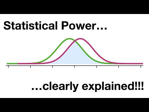
Statistical Power, Clearly ExplainedStatQuest with Josh Starmer

Power, and why it lives on variance

Power = 1 − β is the probability of correctly rejecting H₀ when a specific alternative effect is real — the chance your experiment detects a true effect of a given size. The default is 0.80, meaning you accept a 20% false-negative rate. The non-obvious truth: power is governed by variance, not by the effect size you happen to get. Two experiments with identical true effects have wildly different power if their metrics have different σ². This is why variance reduction (CUPED, L3) is so valuable — halving σ² doubles your effective sample size — and why a high-variance metric like revenue is so much harder to power than a low-variance proxy.

The sample-size equation, derived

Reject H₀ when |Z| > z_1−α/2. For a true effect Δ with standard error SE, the standardised effect is Δ/SE; achieving power 1−β requires Δ/SE = z_1−α/2 + z_1−β. Solve for n with equal allocation and equal variances and you get n = (z_1−α/2 + z_1−β)² · σ² / Δ² per arm. For the canonical α = 0.05 two-sided and power 0.80, the z-scores are 1.96 and 0.84, summing to 2.80, so the coefficient is 2.80² ≈ 7.85. Folding the two-arm variance into one number gives Kohavi’s ubiquitous shortcut: N_total ≈ 16·σ²/Δ².

code

1THE SAMPLE-SIZE / POWER EQUATION, READ FOUR WAYS23  core:  n_per_arm = (z_{1-a/2} + z_{1-b})^2 * sigma^2 / delta^24         at a=0.05 two-sided, power=0.80 -> (1.96 + 0.84)^2 = 7.855         Kohavi shortcut:  N_total ~= 16 * sigma^2 / delta^267  read it for...        you fix...                       you solve for...8  --------------------  -------------------------------  ----------------9  "how long to run?"    a, power, sigma, MDE             n  (-> runtime)10  "what can we rule     a, power, sigma, n_observed      MDE11   out after running?"12  "was the test even    a, sigma, MDE, n_observed        power13   capable?"14  design tradeoff       lower MDE OR more power          bigger n (quadratic!)1516  KEY: n scales with 1/delta^2 -> halving the MDE QUADRUPLES the sample needed.17       balanced 50/50 split minimizes sigma_t^2/n_t + sigma_c^2/n_c -> max power.

Two consequences interviewers test. First, the quadratic: n ∝ 1/Δ², so detecting an effect half as large needs four times the traffic — this is why tiny MDEs are so expensive and why a sensitive metric is worth more than raw users. Second, the balanced-split result: with total sample fixed, equal allocation n_t = n_c = n/2 minimises the variance term and therefore maximises power. Interview angle. “Why 50/50 and not 90/10?” → equal allocation minimises the SE of the difference for a fixed total n; you only deviate to limit exposure of a risky treatment, trading power for safety.

A worked anchor to recite: a 20% baseline conversion, detecting a 5% relative MDE at α = 0.05 / power 0.80, needs on the order of ~11,000 conversions total (SplitMetrics). Convert that to users via the base rate and to runtime via daily traffic — and if the runtime exceeds your release cycle, the design is infeasible and you escalate (L1). Being able to go from MDE → conversions → users → days on a whiteboard, stating every assumption, is exactly what the sample-size question grades.

Confidence intervals: the better default than p

The two-sided 1−α confidence interval for the effect is Δ ± z_1−α/2·SE. It does double duty: it estimates the effect with its uncertainty, and it mirrors the hypothesis test exactly — the test rejects H₀ at level α iff the CI excludes 0. This is why seniors prefer reporting CIs: “the lift is 0.5% ± 0.3% (95% CI)” is far more decision-useful than “p = 0.02,” because it shows magnitude and precision together. For proportions near 0 or 1, prefer Wilson or Agresti-Coull intervals over the naive Wald interval, which has poor coverage in the tails.

The dual is also a warning: a wide CI that includes 0 from an underpowered test is not evidence of no effect — it is evidence you didn’t gather enough data. And the percentile bootstrap, beloved for skewed metrics, does not have the same coverage as a pivotal interval; for clustered online metrics the bootstrap must resample at the experimental unit (user), or it artificially narrows the interval and overstates significance — the clustering trap we hit again under leakage.

Two-sided vs one-sided, and the cost of being wrong

Default to two-sided tests. A one-sided test buys a little power by assuming the effect cannot go the wrong way — but treatments regress metrics all the time, and a one-sided test is blind to a harmful effect, which is exactly what your guardrails are trying to catch. The honest framing of α and power is as business costs: α is the rate at which you ship a no-op believing it works (wasted engineering, possible harm); β is the rate at which you kill a real win (lost opportunity). High-stakes irreversible changes justify a stricter α (0.01); cheap reversible ones can tolerate more. Interview angle. “One-sided or two?” → two-sided unless you can defend why a regression is impossible — and you almost never can.

videoPower Analysis, Clearly ExplainedStatQuest with Josh Starmer paperThe ASA Statement on p-Values: Context, Process, and PurposeWasserstein & Lazar (2016)docsStatistical Analysis of A/B Tests (the z-test, power, CIs, skewness rule)Alex Deng — Causal Inference for the Brave and True notes

Interview prep

The significance-and-power round is a literacy test: interviewers want crisp, correct definitions and the ability to invert the sample-size equation on a whiteboard. The fastest way to lose points is an imprecise p-value sentence or treating significance as effect size. Lead with the definition, then the production implication, then a number.

01“What is a p-value?” → P(data at least this extreme | H₀ true); NOT the probability the hypothesis is true, NOT the effect size (ASA principles 2 & 5).
02“If p = 0.06 and α = 0.05, what do you conclude?” → fail to reject at 0.05; report the effect size + CI; decide whether to extend, rerun, or accept quantified false-positive risk — not “almost significant, ship.”
03“Explain statistical power to a PM.” → the chance we detect a real effect of a given size; 80% means a 20% miss rate — and it’s driven by variance, so a sensitive metric buys power.
04“How do you size an experiment?” → n = (z_{1-a/2}+z_{1-b})^2·σ²/Δ² per arm; fix α, power, σ, MDE; n ∝ 1/Δ² so halving MDE quadruples n.
05“Why a 50/50 split?” → equal allocation minimises the SE of the difference for fixed total n, maximising power; deviate only to cap risky-treatment exposure.
06“CI vs p-value — which do you report?” → the CI on the difference; it shows magnitude + precision and the test rejects iff it excludes 0.
07“Two CIs overlap — significant?” → can’t tell from overlap; test the interval on the difference, which may still exclude 0.
08“One-sided or two-sided?” → two-sided by default; one-sided is blind to harmful effects your guardrails must catch.

Going deeper, the follow-ups probe robustness: “your revenue metric is wildly skewed — is the z-test still valid at n = 5,000?” (maybe not; apply the n > 100·s² skewness rule, cap outliers at the 99th percentile, or bootstrap at the user level); “you have a fixed 2-week runtime — how do you get more power without more traffic?” (variance reduction via CUPED, a more sensitive surrogate metric, or stratification — L3); and “what’s the difference between statistical and practical significance?” (a 0.01% lift on 100M users is significant and trivial; the decision needs effect size, CI, and business value). Name the assumption you’re relaxing in each.

Checkpoint

An interviewer asks you to interpret a result with p = 0.03 at α = 0.05. Which statement is correct?

AThere is a 3% probability that the null hypothesis is trueBIf there were truly no effect, we would see data at least this extreme only 3% of the time — so we reject the null at α = 0.05CThe treatment effect is 3% in magnitude

Checkpoint

Your current design detects a 4% MDE in two weeks. The business now needs to detect a 2% effect. Roughly what happens to the required sample?

AIt doubles — sample size scales linearly with the inverse of the effectBIt’s unchanged if you keep α and power the sameCIt quadruples — n ∝ 1/Δ², so halving the MDE multiplies the sample by four

Checkpoint

A stakeholder says “the treatment and control 95% CIs overlap, so there’s clearly no significant difference.” Best correction?

AAgree — overlapping confidence intervals mean the difference is not significantBThe right object is the confidence interval on the difference, which can exclude 0 even when the two per-arm intervals overlapCRe-run with a one-sided test so the intervals no longer overlap

Checkpoint

Your average-revenue-per-user metric has skewness ~12. Each arm has 3,000 users. What’s the senior concern?

ANone — 3,000 > 30, so the CLT guarantees the z-test is validBThe metric is heavy-tailed; at this n the CLT may not hold, so cap outliers, transform, or bootstrap at the user level before trusting the z-testCSwitch the metric to its log without checking anything else

Checkpoint

A risky redesign could plausibly hurt key metrics. A teammate suggests a one-sided test “to get more power for the win we expect.” Your call?

AUse two-sided — a one-sided test is blind to a harmful effect, which is exactly the risk hereBUse one-sided — the extra power is worth it and the team expects a positive resultCUse one-sided but lower the power target to compensate

Could you define a p-value precisely, invert the sample-size equation on a whiteboard, and report a result as a CI on the difference?

New to itGetting thereConfident

Takeaways

A p-value is P(data this extreme | null true) — never the probability the hypothesis is true, never the effect size.
Power is the chance of detecting a real effect; it lives on variance, so a sensitive metric (or CUPED) buys it.
n = (z+z)²σ²/Δ² per arm; n ∝ 1/Δ² (halve the MDE → 4× the data); 50/50 maximises power.
Report the CI on the difference — it shows magnitude + precision and the test rejects iff it excludes 0.
Default to two-sided; respect the skewness rule (n > 100·s²) before trusting the CLT on heavy-tailed metrics.

Next: randomization, the peeking problem, sequential/always-valid testing, and CUPED variance reduction.

Sources

Free to read · better with Enzo

Learn it with Enzo

Save your progress, answer the checkpoints, and let Enzo quiz you on what you just read.

Continue with Enzo Sign up free