The randomization unit is an architectural decision; SUTVA breaks under network effects; peeking inflates false positives 2-3x; and CUPED halves variance for free. Microsoft hash bucketing, DoorDash switchbacks, Meta cluster randomization, Spotify’s sequential-testing choice, and Bing’s CUPED result — the design decisions that make or break a trustworthy experiment.
Three design decisions the statistics can’t save you from
A perfect t-test on a broken design is still broken. Three design choices decide whether your experiment is trustworthy before any analysis runs: what unit you randomise (and whether SUTVA even holds), how you look at the data over time (the peeking problem), and how much variance you can remove (CUPED). Get the unit wrong and network spillover biases every estimate; peek naively and your 5% false-positive rate becomes 30%+; skip variance reduction and you burn 2× the traffic for the same answer. This is the lesson where the named-company case studies live — Microsoft, DoorDash, Meta, Spotify, Bing.
The randomization unit is an architectural decision
The randomization unit is the thing you flip the coin on. Microsoft’s ExP assigns bucket = hash(user_id + experiment_id) mod 1000 — deterministic, salted with the experiment id so the same user lands in a consistent bucket within an experiment but is re-randomised across overlapping experiments. That salt is the entire trick that makes layered, concurrent experimentation honest: a constant hash would force every experiment to share one already-correlated partition per user. This single design choice is what let ExP scale from Bing across 20+ Microsoft teams.
The unit is bounded by SUTVA — the Stable Unit Treatment Value Assumption — which states one unit’s treatment does not affect another unit’s outcome. Pick a unit too small and SUTVA breaks (network spillover); pick it too large and variance explodes and the test is unpowered. Two real failure modes: randomising at pageview instead of user double-counts users and inflates significance; randomising at session produces correlated outcomes within a user and inflates Type-I error unless you cluster the variance. For multi-device products, randomise on the user_id identity graph, not device cookies, or the same person gets split across arms.
code
1CHOOSING THE RANDOMIZATION UNIT (smallest unit that respects SUTVA)23 unit use when... failure if wrong4 ------------- ------------------------------ ----------------------------5 user (hashed) content/search/streaming; pageview-level double-counts6 one user can't affect another users, inflates significance7 session rarely; needs user-level correlated within-user8 variance clustering outcomes inflate Type-I9 cluster/geo social graphs, marketplaces cross-cluster spillover10 (spillover contained in cluster) biases the estimate11 time (switch- dispatch/pricing/matching where carry-over across periods;12 back) supply rebalances can't run long1314 Microsoft ExP: bucket = hash(user_id + experiment_id) mod 100015 the experiment-id SALT re-randomizes across overlapping tests.
When SUTVA breaks: network effects, switchbacks, clusters
Two-sided marketplaces, social networks, and dispatch systems break the user-randomised A/B because the treatment assigned to user A changes user B’s outcome. DoorDash states it directly: simple A/B tests are ineffective for the Dispatch algorithm because treatment couriers and control couriers draw from the same supply pool — a faster-dispatch treatment evaporates supply that control then can’t use, so a naive user-randomised test measures supply rebalancing, not the algorithm. Their fix is the switchback: alternate the runtime condition for a whole region over time windows, so both arms are observed under the same supply regime. Switchbacks have carry-over between windows and can’t run long, so you analyse within-window.
Meta uses graph cluster randomization for products with strong network effects: partition the social graph into clusters via community detection, then randomise clusters, not users, so spillover is contained inside a cluster and the between-cluster contamination is minimised. The cost is steep — the cluster becomes the unit of inference, so variance rises and you need many clusters, not many users; for very dense graphs the cluster cost can exceed an A/B budget, pushing you toward switchback or quasi-experimental designs. Interview angle. “How do network effects change your design?” → if A’s treatment affects B, don’t user-randomise; cluster at the natural interaction boundary (geo for marketplaces, community for social, time for dispatch) and accept the variance hit.
The peeking problem: why repeated looks lie
A fixed-horizon z-test controls the false-positive rate at exactly α only if you run it once at the pre-planned sample size. The moment you re-check significance as data accumulates and stop when it crosses 0.05, you are running many implicit tests, and the chance of at least one false crossing under the null compounds: roughly 1 − (1 − α)k over k independent peeks. Ten peeks push a nominal 5% to ~40%; continuously monitored naive tests routinely run 2–3× their nominal α in practice. This is the single most common runtime temptation in industry — every GM wants an early read.
code
1PEEKING INFLATES THE FALSE-POSITIVE RATE (naive fixed-horizon z-test)23 peeks (k) approx P(>=1 false positive under null) = 1 - (1 - 0.05)^k4 --------- -----------------------------------------------------------5 1 5% <- the rate you THINK you have6 5 23%7 10 40%8 20 64%9 50 92%1011 "peek until significant, then stop" is optional stopping -> the estimate is12 also biased upward (you stop on lucky upswings). Tightening the threshold13 (0.01, then 0.005) only DELAYS the inflation; it does not fix it.1415 fixes: pre-commit a stop date and look once; OR use a sequential method that16 is valid under continuous monitoring (group-sequential, mSPRT, CS).
Optional stopping does a second damage beyond false positives: it biases the effect estimate upward, because you stop precisely on the random upswings. So peeked-and-stopped experiments both over-reject the null and overstate the lift when they do. The naive defenses don’t work: tightening the threshold over time (0.01, then 0.005) only postpones the inflation, and “we only peeked a few times” still compounds. Interview angle. “A GM demands an early read at day 3 — what do you do?” → either pre-commit to a fixed horizon and refuse to act on interim looks, or switch the whole experiment to an always-valid method that earns the right to peek.
Sequential & always-valid inference: earning the right to peek
Three frameworks let you look early without breaking α — and they converge at the planned endpoint but diverge sharply in how they absorb unplanned looks. (1) Group-sequential with alpha-spending (Lan-DeMets): pre-pick a max sample and a small number of interim looks; an alpha-spending function budgets the total Type-I error across those looks, each using a stricter threshold. Most powerful when the max sample size is known; cannot absorb unbounded peeks. (2) Always-valid / mSPRT (Johari, Pekelis, Walsh 2015): a mixture sequential probability ratio test that rejects when the mixture likelihood Λ ≥ 1/α, valid at any stopping time; most powerful when the horizon is unknown. (3) Confidence sequences (Howard, Ramdas, McAuliffe, Sekhon 2021): time-uniform intervals with P(Lt ≤ μ ≤ Ut for all t) ≥ 1−α, distribution-free and valid at every stopping time.
code
1THREE SEQUENTIAL FRAMEWORKS (all valid under monitoring; pick by horizon)23 framework best when... peeking behavior4 -------------------- ------------------------ --------------------------5 fixed-horizon z pre-planned, no monitoring Type-I inflates per peek6 group-sequential max N known, few interim alpha spent across PLANNED7 (alpha-spending) looks (efficacy/futility) looks; not robust to extra8 always-valid / mSPRT horizon unknown, streaming Type-I held at ANY stop9 confidence sequences distribution-free, any t time-uniform coverage1011 At the pre-planned endpoint, mSPRT/GST collapse toward the standard z-test,12 so you recover (nearly) full power. Spotify (2023) DEFAULTS to group-sequential13 because their max sample size is usually knowable -> it keeps the most power14 at the planned endpoint; AVI/mSPRT is reserved for streaming/exploratory15 platforms with no known horizon.
The choice is by horizon knowledge, not by form. Spotify’s 2023 engineering write-up is the canonical industry framing: they default to group-sequential tests with alpha-spending because their experiments usually have a knowable maximum sample size and GST retains the most power at the planned endpoint, reserving always-valid inference for streaming/exploratory contexts without a fixed horizon. The cost of always-valid is a modest power hit relative to a perfectly-planned fixed test — you’re buying the freedom to stop early in exchange. Interview angle. “Bayesian sequential vs mSPRT?” → both let you monitor continuously; mSPRT controls frequentist Type-I at any stop via a mixture prior, while a Bayesian approach reports posterior probabilities and needs a genuine prior — name the guarantee each gives.
CUPED: cut variance in half, double your sensitivity
CUPED (Controlled-experiment Using Pre-Experiment Data) is the highest-leverage variance reduction in the toolkit. For each unit, adjust the outcome using a pre-period covariate X: Ycuped = Y − θ·(X − μX) with the optimal θ = Cov(Y,X)/Var(X). The result is Var(Ycuped) = (1 − ρ²)·Var(Y), where ρ is the correlation between the pre-period covariate and the in-experiment metric. If ρ = 0.7, variance drops by half — equivalent to doubling your sample size for free. Bing’s original result (Deng, Xu, Kohavi, Walker, WSDM 2013) reported ~50% variance reduction, i.e. doubling experiment sensitivity.
code
1CUPED VARIANCE REDUCTION (Y_cuped = Y - theta*(X - mu_X), theta = Cov(Y,X)/Var(X))23 Var(Y_cuped) = (1 - rho^2) * Var(Y) rho = corr(pre-period X, in-exp Y)45 rho variance reduction effective sample-size multiplier6 ----- ------------------ --------------------------------7 0.3 9% ~1.1x8 0.5 25% ~1.3x9 0.7 51% ~2.0x <- Bing's reported ~50% (doubles sensitivity)10 0.9 81% ~5.3x1112 unbiased IFF pre-period E[X_t] - E[X_c] = 0 (guaranteed by randomization).13 estimate theta on the WHOLE population, not per arm (per-arm introduces a14 treatment x pre-exposure interaction and biases the estimate).
CUPED is unbiased precisely because randomisation guarantees the pre-period means are equal across arms in expectation (E[Xt] − E[Xc] = 0), so the adjustment only removes pre-existing user-level variance, never the treatment effect. The best covariate is usually the same metric measured in the pre-period (high ρ). Three failure modes to know: choosing a low-correlation covariate wastes the technique; estimating θ per arm introduces a treatment×pre-exposure interaction and biases the result (estimate it on the pooled population); and using a covariate the treatment can affect in the pre-window violates the parallel-pre-trend assumption. CUPED also stacks with sequential testing — the smaller SE lowers the per-peek inflation and shrinks the always-valid interval. Extensions (CUPAC, in-experiment covariates) push further.
The design round tests whether you treat the experiment’s structure — unit, monitoring, variance — as first-class. Interviewers reward naming the failure mode each choice guards against: SUTVA for the unit, Type-I inflation for peeking, and the (1−ρ²) gain for CUPED. Lead with the mechanism and a named-company example.
01“What unit do you randomise on, and why?” → smallest unit respecting SUTVA; user-hash with experiment-id salt for content; cluster/geo/time when interference is real.
02“How do network effects change your design?” → if A’s treatment affects B, don’t user-randomise — switchback (DoorDash dispatch) or graph clusters (Meta social); the cluster becomes the unit of inference.
03“What is the peeking problem?” → repeated significance checks compound false positives toward 1−(1−α)^k (10 peeks ≈ 40%) and bias the estimate upward via optional stopping.
04“How do you let people stop early safely?” → group-sequential with alpha-spending (known max N) or always-valid/mSPRT (unknown horizon); pre-commit the method.
05“Group-sequential vs always-valid — which and when?” → GST when max N is known (most power at the endpoint, Spotify’s default); mSPRT for streaming/unknown horizon.
06“How do you get more power without more traffic?” → CUPED: Var drops by (1−ρ²); ρ=0.7 halves variance ≈ doubles sample size (Bing’s ~50%).
07“Why is CUPED unbiased?” → randomisation makes pre-period means equal in expectation, so the adjustment removes pre-existing variance, not the treatment effect — estimate θ on the pooled population.
08“A GM wants a day-3 read on a 2-week test — what do you say?” → interim looks on a fixed-horizon test inflate α; either commit to the horizon or run an always-valid design that earns the peek.
Going deeper, the follow-ups probe the edges: “how do you pick the CUPED covariate and what if the treatment touches it pre-period?” (use the same metric pre-experiment for max ρ; if the treatment can influence the covariate window, the parallel-pre-trend breaks and CUPED is biased); “switchback carry-over — how long a window?” (long enough for the system to reach steady state under each condition, analysed within-window, accepting reduced power); and “can you combine CUPED and sequential testing?” (yes — they stack; the smaller SE tightens the always-valid interval). Name the assumption each technique rests on.
Checkpoint
You’re A/B testing a new courier-dispatch algorithm in a two-sided delivery marketplace. Treatment couriers are dispatched faster. What design issue dominates?
ANone — user-level randomisation of couriers is fine if the split is 50/50BSUTVA is violated by supply spillover; use a switchback that alternates the condition for a whole region over time windowsCJust increase the sample size until the difference is significant
A teammate has been checking the experiment dashboard every day for two weeks and wants to stop now that p just dropped below 0.05. What’s the problem?
AOptional stopping — daily peeks compound the false-positive rate well above 5% and bias the effect upward; you needed a fixed horizon or a sequential methodBNothing — once p < 0.05 the result is significant regardless of how many times you lookedCThe threshold should have been 0.01 from the start, which would have made the daily peeks fine
Your experiments almost always have a known maximum sample size, but the team wants the option to stop early for clear wins or losses. Best framework?
AAlways-valid mSPRT, because it’s valid at any stopping timeBJust use a fixed-horizon test and forbid early stoppingCGroup-sequential with alpha-spending — most powerful at the planned endpoint when max N is known, with budgeted interim looks (Spotify’s default)
You have a strong pre-period signal: each user’s pre-experiment value of the metric correlates ρ ≈ 0.7 with their in-experiment value. What does CUPED buy you?
AAbout a 50% variance reduction — roughly doubling effective sample size and sensitivityBNothing useful unless ρ is above 0.95CA larger measured treatment effect, because the adjustment amplifies the signal
An analyst computes the CUPED adjustment θ separately within the treatment arm and within the control arm. What’s the senior concern?
AIt’s the correct approach — per-arm θ tailors the adjustment to each groupBθ must be estimated on the pooled population; estimating it per arm introduces a treatment×pre-exposure interaction that biases the estimateCIt doesn’t matter as long as both arms use the same covariate
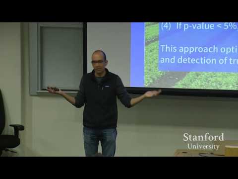 Peeking at A/B Tests — Why It Matters and What to Do About ItStanford Seminar (Optimizely)
 Always Valid Inference: Continuous Monitoring of A/B TestsData CouncilpaperImproving the Sensitivity of Online Controlled Experiments by Utilizing Pre-Experiment Data (CUPED)Deng, Xu, Kohavi & Walker (WSDM 2013)paperAlways Valid Inference: Bringing Sequential Analysis to A/B TestingJohari, Pekelis & Walsh (arXiv)articleChoosing a Sequential Testing Framework — Comparisons and DiscussionsSpotify EngineeringarticleSwitchback Tests and Randomized Experimentation Under Network Effects at DoorDashDoorDash Engineering